
Overview of millimeter wave radar
Millimeter wave radar is an important sensor used in obstacle detection for mobile robots. Millimeter-wave radar is now being used in commercial automobiles, especially luxury cars, and is said to become an indispensable sensor for automated driving systems and driver assistance systems. In addition to automobiles, they are also installed in mobile robots such as drones and transport equipment (AGVs, AWRs). They are also used in partial robotic functions, such as the automatic stop function of heavy machinery (construction equipment) such as bulldozers.
Millimeter wave radar is a sensor that uses radio waves (electromagnetic waves) called “millimeter waves” to detect the distance of obstacles. A millimeter wave is a radio wave with a wavelength of several millimeters (1 mm to 10 mm). The name “millimeter wave” is derived from the fact that it has a wavelength of several millimeters. In terms of frequency, it is in the range of 30 GHz to 300 GHz. However, as with other wavelength bands, there is no strict definition; for example, radio waves at 20 GHz are sometimes called millimeter waves.
Radar using radio waves with longer wavelengths (lower frequencies) than millimeter-wave waves is widely used in applications such as obstacle detection for ships and airplanes and rain cloud radar.
Starting from the next section, we will touch on the basic knowledge and technology involved in millimeter wave radar to get a general picture.
Basic functions and configuration of millimeter wave radar
Millimeter wave radar is a type of ranging sensor. It uses the distance information obtained to determine if there is an obstacle. For example, if the measured distance to an object is less than 100m, it is considered to be an obstacle. There are two patterns: one is to measure the distance to the obstacle in each direction (e.g., three directions), and the other is to create distance image data by dividing the measurement direction into a mesh of vertical and horizontal directions.
A millimeter wave radar consists of a transmitting function to emit radio waves and a receiving function to detect them. The basic configuration diagram is shown below (detailed configuration is described later). An “antenna” is used to transmit and receive radio waves, including millimeter waves. On the transmitter side, a transmitter circuit consisting of a power amplifier (PA) and other components is connected to the antenna for transmission. By sending a signal waveform (in the form of a sine wave) from the power amplifier to the antenna, the antenna emits radio waves. On the receiving side, a receiving circuit consisting of a low-noise amplifier (LNA) and other components is connected to the antenna for reception. The antenna detects the radio wave and converts it into a voltage signal, and the low-noise amplifier amplifies the signal level and passes it to the subsequent signal processing circuit.
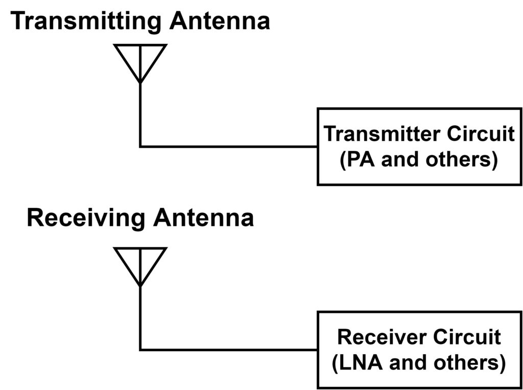
The basic operating principle of millimeter wave radar is based on the same idea as that of general wireless communication systems, and the circuit configuration is similar. Some wireless communication systems share the same antenna for transmission and reception and use them separately in time (time division), but millimeter wave radar often has separate antennas in the process of devising ways to increase spatial resolution (angular resolution).
Millimeter-wave radar estimates the distance to an object by irradiating millimeter-wave radio waves at the object, detecting the radio waves that bounce back, and measuring the time taken for the round trip. The distance can be calculated by multiplying the time by the speed. Since radio waves are a type of electromagnetic wave similar to light (visible light), the speed of millimeter waves is the speed of light. Assuming that the distance to the object is \(R\)(round trip distance is \(2R\)), the time is \(\Delta T\), and the speed of light is \(c\), the following equation is established, and the distance \(R\) is now obtained.
$$~~2R = \Delta T \times c$$
$$~~R = \frac{\Delta T \times c}{2}$$
This method of calculating distance from the time of flight of radio waves, etc. is called TOF (Time of Flight). Some methods do not apply, but basically millimeter wave radar is classified as a type of TOF sensor.
Frequency of millimeter wave radar
The three main frequency bands available for millimeter-wave radar are the 76 GHz (77 GHz), 79 GHz, and 24 GHz bands. As with general wireless communications (e.g., WiFi is allocated the 2.4 GHz and 5 GHz bands), the frequencies available are determined in detail. The wavelengths of 76 GHz and 79 GHz are about 4 mm, and the wavelength of 24 GHz is about 12.5 mm. The 24 GHz wavelength is sometimes called “quasi-millimeter wave” because it is not strictly included in the millimeter wave definition of 1 to 10 mm.
Each of the three frequency bands has a range of frequencies: 76 GHz from 76.0 to 77.0 GHz, 79 GHz from 77.0 to 81.0 GHz, and 24 GHz from 24.05 to 24.25 GHz. These ranges are determined by laws and regulations of each country, and are managed by government agencies. (In Japan, the Ministry of Internal Affairs and Communications, and in the U.S., the Federal Communications Commission, have jurisdiction. The reason for this is to consider the space that carries radio waves as a shared asset of the people (humanity) and to ensure that it can be used efficiently without becoming a lawless zone. This way of thinking is possible because of the physical (mathematical) nature of radio waves, which allows the receiver to sort out the transmitted information even if multiple radio waves are flying in the same place, as long as the frequencies are separated.
The first reason for having a wide range of frequencies is that it is impossible to control the frequency at a single point in the real world. (This is similar to the difficulty in controlling a voltage value of 1.500000000V or so.) The second reason is that information can be transmitted more efficiently with a wider range of frequencies. For example, a single frequency band can be further divided into multiple detailed frequency ranges called channels, and different information can be transmitted on multiple channels simultaneously. The larger the frequency range (the wider the bandwidth), the higher the communication speed and the accuracy of ranging. In this sense, the 79 GHz band is the most accurate of the three frequency bands because it can use the 4 GHz range of 77 to 81 GHz.
Advantages and disadvantages of millimeter wave radar
One of the greatest advantages of millimeter wave radar is that its range-finding performance is not affected by weather conditions when installed in robots that move around outdoors, such as self-driving cars. For example, when using visible light to see ahead like the human eye, it is difficult to find obstacles when rain, fog, or snow occurs. Visibility at night is also greatly impaired with visible light (even with car headlights on). Compared to the electromagnetic waves used in other ranging sensors such as visible light and infrared rays, millimeter waves are relatively less susceptible to attenuation caused by moisture such as rain, making it easier to maintain the ranging function even in bad weather.
Compared to radio waves with longer wavelengths (lower frequencies), the shorter wavelengths have the advantage that the size of the antenna can be reduced. It is said that in order to transmit and receive radio waves efficiently, the size of the antenna needs to be larger than half the wavelength (λ/2), and millimeter waves with short wavelengths allow for smaller antennas. The short wavelength of millimeter waves also has the advantage of reducing the distance resolution and spatial resolution, which in principle can improve the accuracy of distance measurement sensors.
The disadvantage is that the spatial resolution (angular resolution) is poor (large) compared to other ranging sensors such as stereo cameras and LiDAR. This will be discussed later. Another disadvantage is that when used for automated vehicles, noise called clutter from objects other than the target object, such as guardrails, becomes larger.
Principle of millimeter wave radar
As mentioned above, millimeter wave radar is a type of TOF sensor, and there are two main types of radar systems in common use. The two most commonly used methods are the “pulse radar” and the “FMCW radar”. The pulse method has a simple principle and a relatively simple circuit configuration. The FMCW method is widely used in automobile driver assistance systems and automatic driving systems because it can measure the distance to an object as well as the relative movement speed of the object.
Pulse radar
The pulse radar emits millimeter waves in pulses. The pulsed radio waves bounced back from the object are received, and the distance to the object is estimated from the time difference. The formula for the relationship between distance and time is as described above. The following figure shows the image of the transmitted and received pulses.
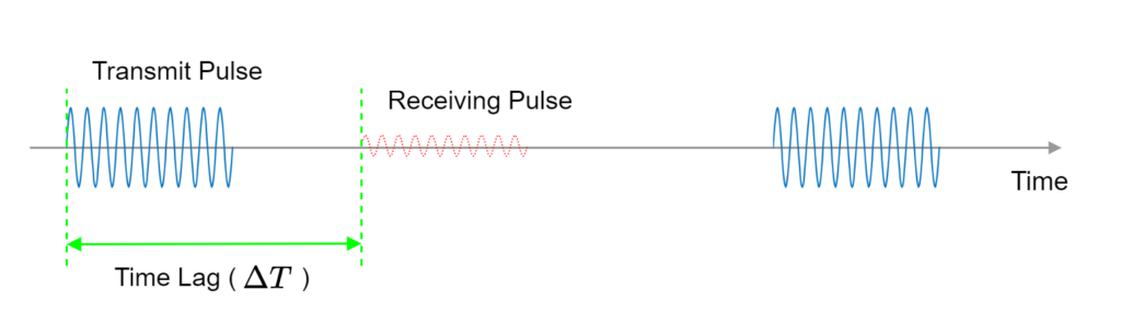
This figure shows the time on the horizontal axis and the intensity of the radio wave on the vertical axis. To make it easier to see, the number of sine waves in a single pulse is set to 10 periods in this figure, but in reality, many more sine waves are included. In addition, the power (strength) of the received radio wave is many orders of magnitude smaller than the power of the transmitted wave, making it very weak. If this were represented realistically in the figure, the received pulse would not be visible at all, so it has been exaggerated and drawn larger.
The reason for including multiple sine waves in a single pulse is to increase the sensitivity of reception; a single sine wave is more difficult to separate from noise. It is intuitive that the more sine waves there are, the easier it is to detect.
FMCW radar
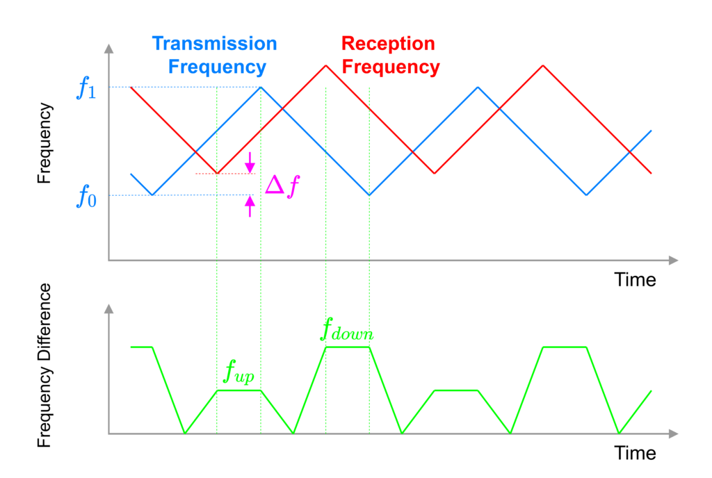
The FMCW method is a method in which the frequency of the radiated radio waves is continuously and gradually changed. FM stands for Frequency Modulation, a method of expressing transmitted information in terms of frequency changes. CW is an acronym for continuous wave, which means that the radio waves are output continuously without interruptions as in the pulse method. The following figure shows a graph showing the time variation of the frequency of the radiated radio wave. The radio wave that hits an object and bounces back to be received is delayed by the time difference according to the distance, and takes the same form.
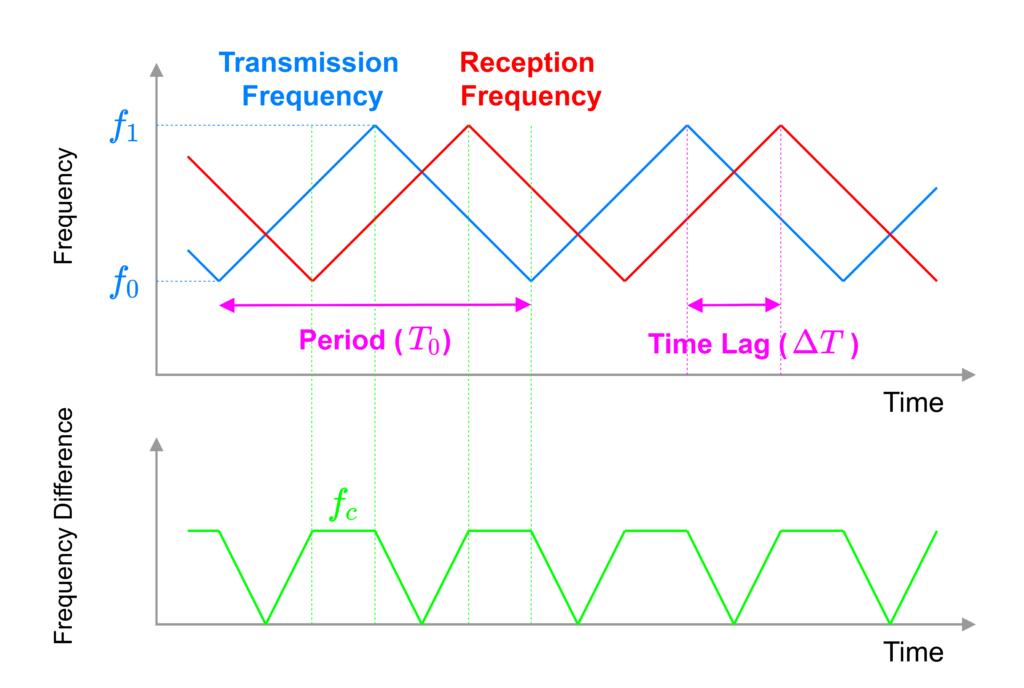
As shown in the graph at the bottom of the figure, calculate the absolute value of the difference between the transmit and receive frequencies, and find the time value (\(f_c\)) at which it is constant. This corresponds to the time difference between transmission and reception, and the following equation is established.
$$~~\Delta T = \frac{T_0 \times f_c}{2(f_1-f_0)}$$
For example, if you find a right triangle with base \(T_0/2\) and a right triangle with base \(\Delta T\), and the slopes of each are equal, you will get the following equation.
$$~~\frac{(f_1-f_0)}{(T_0/2)} = \frac{f_c}{\Delta T}$$
Then, based on the principle of the TOF sensor, the distance \(\Delta T\) to distance \(R\) can be obtained.
$$~~R = \frac{ΔT \times c}{2} = \frac{T_0 \times f_c}{2(f_1 – f_0)} \times c \times \frac{1}{2}$$
$$~~~~= \frac{T_0 \times f_c \times c}{4(f_1 – f_0)}$$
A waveform with a continuously changing frequency is called a “chirp waveform” or “chirp signal”. This term is also commonly used in other technical fields besides radio waves. A chirp waveform can be expressed as a graph with intensity on the vertical axis, as shown in the figure below.
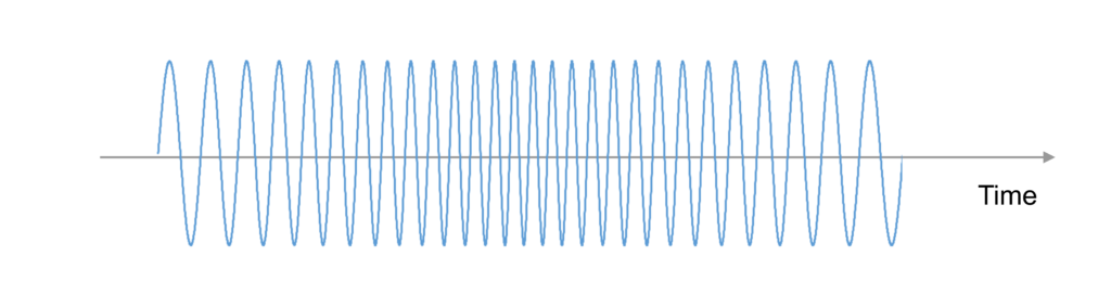
The waveform looks like a shortening or lengthening of the period. Note that the frequency change is drawn more exaggeratedly than it actually is. In addition, the range of frequencies to be changed should be within the frequency range specified by laws and regulations as described above.
We mentioned earlier that the FMCW method has the feature of being able to determine not only the distance to an object, but also its relative velocity. In order to understand this feature, we need to consider the graph of the frequency waveform a little more realistically. Since radio waves are a type of “wave,” when the object radiating the wave and the object receiving the wave move at different speeds, the “Doppler effect” occurs and the frequency changes. In other words, the further the object moves away from the robot (car) equipped with the radar, the lower the received frequency becomes, and conversely, the closer the object gets, the higher the received frequency becomes. By detecting this change in frequency due to the Doppler effect, the relative velocity can be determined. The following figure shows the waveform of the frequency when the Doppler effect is taken into account. This figure assumes that the speed of the object in front is slower than the radar itself and is approaching.
The amount of shift in frequency due to the Doppler effect \(f_d\) is related to the relative velocity between the radar and the target by the following formula.
$$~~f_d = \frac{2 \times v \times f_c}{c}$$
This formula can be derived from the formula for the Doppler effect of electromagnetic waves. Assuming that the frequency of the radio wave to be transmitted is \(f_a\), the frequency to be received is \(f_b\), the relative velocity between the radar and the target is \(v\), and the speed of light is \(c\), the formula is as follows.
$$~~f_b = \frac{\sqrt{1-(\frac{v}{c})^2}}{(1-\frac{v}{c})} f_a$$
Note that the equation is different from the Doppler effect in the case of sound waves. In the case of electromagnetic waves, the speed at which the signal travels is the “speed of light. Based on the theory of relativity, the speed of light has the curious property that it remains constant regardless of the speed of the observer. (In the case of sound waves, the speed of sound, the speed at which the signal travels, depends on the speed of the observer. Because of this property, the form of the equation is slightly different compared to sound waves.
We will transform this equation by approximate calculation using Taylor expansion. The relative velocity \(v\) is approximated by assuming that it is sufficiently small compared to the speed of light, i.e. \(v/c \ll1\).
$$~~f_b = \frac{\sqrt{1-(\frac{v}{c})^2}}{(1-\frac{v}{c})} f_a$$
$$~~~~\simeq \sqrt{1-\left(\frac{v}{c}\right)^2}\left(1+\frac{v}{c}\right)f_a$$
$$~~~~\simeq \left(1-\frac{1}{2} \left(\frac{v}{c}\right)^2\right)\left(1+\frac{v}{c}\right)f_a$$
$$~~~~\simeq \left(1-\frac{1}{2} \left(\frac{v}{c}\right)^2 + \frac{v}{c} -~ \frac{1}{2} \left(\frac{v}{c}\right)^3\right)f_a$$
$$~~~~\simeq \left(1 + \frac{v}{c}\right)f_a$$
The amount of change in frequency \((f_b – f_a)\) is as follows.
$$~~f_b – f_a \simeq \left(1 + \frac{v}{c}\right)f_a- f_a = \frac{v \times f_a}{c}$$
In the case of radar, the Doppler effect (Doppler shift) occurs twice, from radar to object and from object to radar, so the amount of frequency change is doubled. In other words, the amount of frequency change \(\Delta f\) that is finally observed at the receiving end of the radar is as follows.
$$~~\Delta f = \frac{2v \times f_a}{c}$$
This \(\Delta f\) can be obtained by measuring \(f_{up}\) and \(f_{down}\) in the graph below the previous figure.
$$~~\Delta f = \frac{f_{down}-f_{up}}{2}$$
From this, the relative velocity \(v\) can be obtained.
$$~~v = \frac{\Delta f \times c}{2f_a} = \frac{(f_{down} – f_{up}) \times c }{4 f_a}$$
Since \(f_a\) is the frequency generated in the transmitter circuit, it is known. Since the speed of light is also known, if we can measure \(f_{down}\) and \(f_{up}\), we can determine the relative velocity \(v\). As described above, the feature of the FMCW method is that it can measure the relative velocity as well as the distance.
By the way, to calculate the distance taking into account the Doppler effect, you can use the following formula to find fc, which is used to calculate the distance.
$$~~f_c = \frac{f_{down} + f_{up}}{2}$$
Circuit configuration (FMCW radar)
The circuit configuration of the FMCW system is shown below. The basic configuration is the same as that of a general wireless communication system, but the difference is that the chirp signal of the transmission is also used as is on the receiving side. The configuration diagram is shown in the figure below.
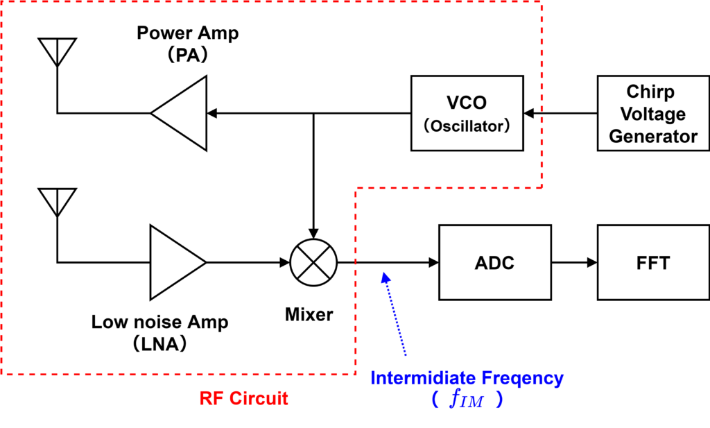
The transmitter side consists of an oscillator that generates the chirp signal, a power amplifier that amplifies the power so that the antenna can output a radio wave of sufficient strength, and an antenna. The oscillator that generates the sine wave is a “VCO (Voltage Controlled Oscillator)” that has the ability to change its frequency according to the input voltage. The VCO has the ability to control the frequency according to the input voltage, so if the input voltage is increased or decreased linearly, a chirp waveform can be obtained.
The received radio wave is first converted into a voltage signal at the “antenna”. The power of this radio wave is very weak and the voltage value is small. This voltage signal is effectively amplified with low noise using an amplifier called “LNA (Low Noise Amplifer)”. This signal can be a sine wave with a frequency of 76 GHz, for example. You transmit and receive radio waves at this frequency to carry information. In this sense, the frequency of the radio wave is called the “carrier”. (This is the same meaning as the term “carrier” used to refer to cell phone companies such as Docomo. The circuit that processes at the frequency of the carrier is called the “RF circuit” or “high frequency circuit”. The frequency of the carrier is also called RF, which stands for Radio Frequency, which is exactly what it sounds like.
From this carrier frequency, the frequencies of \(f_{down}\) and \(f_{up}\) shifted by the Doppler effect are extracted. There is a famous technique called “FFT (Fast Fourier Transform)” to measure the frequency of a sine wave, and FFT is also used in millimeter wave radar. Since the FFT targets a sampled digital signal (converted into equally spaced discrete time data), it is necessary to AD convert the RF signal, which is an analog signal. The sampling rate of the ADC that performs the AD conversion is several Gsps (several GHz) at most, so it cannot handle high-frequency sine waves such as 76 GHz. (According to the sampling theorem, a sine wave of 76 GHz requires a sampling rate of 152 GHz, twice as high.)
Therefore, based on the general method of wireless communication systems, the frequency of the sine wave is once lowered by a mixer, and then AD conversion is performed. The mixer is an analog circuit that multiplies signals (waveforms) together, as you can see from the symbol in the figure. In the receiving part of the millimeter wave radar, the sine wave of transmission and the sine wave of reception are input. If the frequency of transmission is \(f_a\) as shown in the above formula and the frequency of reception is \(f_b\), the waveform at the output of the mixer will be as shown in the formula below. This is due to the trigonometric function formula.
$$~~sin(~ 2 \pi f_a t ~) \times sin(~ 2 \pi f_b t ~) $$
$$~~~~=\frac{1}{2}\left(~ sin(~ 2 \pi ~(f_a + f_b)~ t ~) + sin(~ 2 \pi ~(f_b -f_a)~ t ~)~\right)$$
A sine wave with a frequency of \((f_a + f_b)\) in the first term is about twice the frequency of the RF frequency. This is too large a frequency for even an RF circuit to process, and the signal is attenuated to become very small. In effect, the effect of a low-pass filter is at work. As a result, only the sine wave at the frequency of the second term \((f_b – f_a)\) remains, which is effectively the output of the mixer. \((f_b – f_a)\) is the frequency range of the chirp signal, which in the case of the 76 GHz band is less than 1 GHz, a level that allows AD conversion. Thus, in wireless communication systems, it is common to reduce the frequency of the sine wave to an intermediate frequency (IF, Intermediate Freqency) so that the necessary arithmetic processing can be performed relatively easily. (This is sometimes referred to as a superheterodyne system. Now we can measure the difference between the transmit and receive frequencies, \((f_b – f_a)\).
Performance of Millimeter Wave Radar
There are two important performance indicators for distance sensors: distance resolution and angular resolution. These are “distance resolution” and “angular resolution”. Resolution here means that when two objects are in the field of view, how far apart are the two objects so that they can be recognized as two separate objects instead of one? It is like human “eyesight”. The definition of human visual acuity is angular resolution, and visual acuity of 1.0 corresponds to a resolution of 1 minute (1/60 degree).
Distance resolution
The theoretical value of the distance resolution of the FMCW millimeter-wave radar can be derived as follows. First, we recall that the distance \(R\) formula we derived before considering the Doppler effect was proportional to \(f_c = f_b – f_a\). From this relationship, we can see that the resolution of \(f_c\) determines the resolution of \(R\). \(f_c\) is measured by FFT, which is roughly equivalent to counting the number of sine waves contained in a given period of time. The smallest unit of number is one. In other words, if there is no more than one sine wave of frequency \(f_c\) in the frequency measurement period \(T_0/2\), then \(f_c\) is recognized as zero. Or, even if the distance of the object to be detected changes in the real world, the change in distance cannot be recognized unless there is a difference of at least one sine wave. The mathematical expression of this is as follows. We use the fact that the number of sine waves can be obtained by multiplying the frequency by the period.
$$~~f_b \times T_0 – f_a \times T_0 = \frac{fc_ \times T_0}{2} > 1$$
$$~~f_c > \frac{2}{T_0}$$
The relation between the distances \(R\) and \(f_c\) are the following.
$$~~f_c = \frac{R \times 4(f_1 – f_0)}{T_0 \times c}$$
So, substituting the above equation, we get the following.
$$~~\frac{R \times 4(f_1 – f_0)}{T_0 \times c} > \frac{2}{T_0}$$
$$~~R > \frac{c}{2(f_1 – f_0)} $$
This is the equation that expresses the resolution of the distance. \(f_1 – f_0\) is sometimes called “bandwidth” in the sense of the width of the frequency used for wireless communication. The maximum bandwidth available in the 76GHz band is 1GHz, which gives a distance resolution of 0.15m (15cm), and the maximum bandwidth in the 79GHz band is 4GHz, which gives a distance resolution of 3.75cm. Both of these levels are sufficient for automotive applications. Although 15cm resolution is not enough for parking operation, it is enough for the performance required for millimeter wave radar, since ultrasonic sensors can be used to measure the distance more precisely at short distances.
In reality, this number may be higher due to the addition of performance degradation factors such as noise from reflections from objects other than the target object, circuit accuracy, and noise. The actual distance resolution of millimeter-wave radar products is likely to be in the range of several cm to several tens of cm.
Angular resolution
In order to detect the horizontal or vertical position of an object with millimeter wave radar, it is necessary to have multiple transmitting and receiving antennas in a row. As shown in the figure below, the position is estimated by using the fact that the “phase” of the radio wave reflected from the object and returned by each antenna is different. The technology and configuration of multiple transmitting and receiving antennas, each handling a different signal, is called MIMO (Multi Input Multi Output).
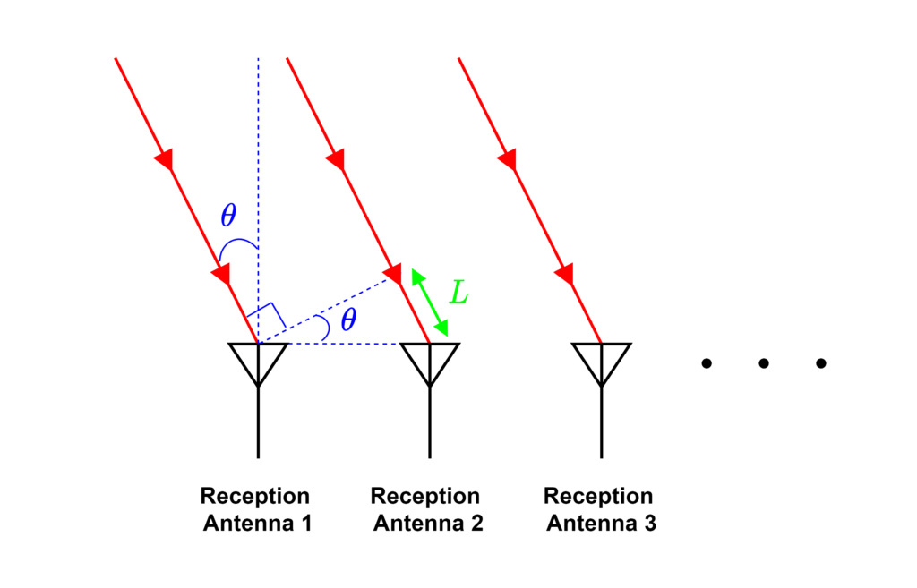
In rangefinding sensors, horizontal and vertical positions are expressed as angles. Therefore, we will first organize the method of calculating the angle by referring to the previous figure. The angle of the direction of travel of the reflected wave from the object is \(\theta\), the distance between the receiving antennas is \(d\), the phase difference is \(\phi\), and the wavelength of the radio wave is \(\lambda\). \(\theta\) is the angle information we want to find. Using these variables, the length of \(L\) in the figure can be expressed as follows. This is a simple trigonometric function and geometry calculation.
$$~~L = d~sin(\theta)$$
The relationship between this and the phase difference is shown below.
$$~~\phi = \frac{2 \pi \times L}{\lambda} $$
Substituting (L) into the above equation, we get the following.
$$~~\phi = \frac{2 \pi \times d~sin(\theta)}{\lambda} $$ So, \(\theta\) is obtained as follows.
$$~~\theta = sin^{-1}\left( \frac{\phi \times \lambda}{2 \pi d}\right)$$
Next, we consider the angular resolution. As shown in the previous equation, the angle \(\theta\) is obtained from the phase difference \(\phi\). There are several ways to measure the phase difference, but we will assume the case where FFT is used. the most commonly used output format of FFT is a graph with frequency on the horizontal axis and intensity on the vertical axis, but based on the principle of Fourier transform, a graph with phase on the horizontal axis and intensity on the vertical axis can also be output. (If the target of the transformation is a superposition of infinite sine waves, the information calculated by the Fourier transform is “reversible” to the waveform information in the time axis direction, and includes phase information. The number of data points in the phase direction in the FFT is determined by the number of antennas (\(N\)). Since the phase range is 0 to \(2\pi\)(0 to 360°), the resolution of the phase difference \(\Delta \phi\) is as follows.
$$~~\Delta \phi = \frac{2 \pi}{N}$$
From the above equation, the relationship between \(\Delta \phi\) and angular resolution \(\Delta \theta\) is as follows.
$$~~\frac{d \phi}{d \theta} = \frac{2 \pi d~cos(\theta)}{\lambda}$$
$$~~\frac{\Delta \phi}{\Delta \theta} = \frac{2 \pi d~cos(\theta)}{\lambda}$$
$$~~\Delta \theta = \frac{\Delta \phi \times \lambda}{2 \pi d~cos(\theta)} $$
$$~~~~= \frac{2 \pi}{N} \times \frac{\lambda}{2 \pi d~cos(\theta)}$$$$~~= \frac{\lambda}{N \times d~cos(\theta)}$$
In general, the distance between receiving antennas \(d\) is often set to about \(\lambda/2\), so we assume \(d = \lambda/2\).
$$~~\Delta \theta = \frac{2}{N~cos(\theta)}[rad]$$
This is the formula for angular resolution. The unit of this equation is radians (rad). The angular resolution in the forward direction (\(\theta=0\)) is the following.
$$~~\Delta \theta = \frac{2}{N}$$
For example, if there are 16 receiving antennas, the angular resolution is 0.125 rad (7.2°).
From this equation, we can see that the more antennas we have, the better the angular resolution will be. Since it is difficult to physically increase the number of antennas, it is possible to set up multiple transmit antennas and hypothetically increase the number of receive antennas. This is called MIMO.
The angular resolution of actual millimeter-wave radar products is about 1° at the highest accuracy. For example, if an obstacle is 100 meters in front of you, 1° corresponds to 1.7 meters in the horizontal (vertical) direction. In the case of a car, this is about the width of a slightly larger car. This is considered sufficient for auto cruising on highways, following the car in front. On the other hand, on ordinary roads, where obstacles become more complex, this is not enough. 0.1° or so (0.1 to 0.2 in human eyesight) is what you want. Millimeter wave radar is expected to be used for detecting distant obstacles since it is not easily affected by weather conditions, but it is said that it will be necessary to use another ranging sensor such as LiDAR in combination with it due to its low angular resolution.
